
ALL MATERIAL COPYRIGHT KEVIN SCOTT 2011. LINKS TO THIS SITE ARE WELCOME BUT DO NOT COPY MATERIAL FROM THIS SITE TO ANY OTHER WEBPAGE.


If you find this site useful, please support it by making a donation of $1 to help maintain and develop it. Click on the PAYPAL DONATE button to do this safely. But there is no obligation - please avail yourself of the information and facilities of the site at no charge.
A traditional mercury barometer can be regarded as an absolute instrument: if the bore is reasonably large, if the glass tube and the mercury are clean,
the Torricellian vacuum good and the engraved scales accurate, then the instrument will read the prevailing atmospheric pressure from the point of its construction
without reference to any other atmospheric data source. It is thus a primary instrument as opposed to other barometric instruments: electronic, aneroid and sympiesometric.
As these primary mercury-containing instruments give way to non-mercurial, secondary instruments, the need for a method of absolute calibration arises. For many practical purposes,
of course, the prevailing atmospheric pressure can be obtained from local weather stations via the Internet or indeed from a mercury barometer in good order if such be available. However,
in principle, and in sometimes in practice, the absolute calibration of a secondary instrument becomes desirable. This paper describes such a method which when carefully applied,
can result in the absolute calibration of a barometer to 0.1mB precision or better.
The subject of the particular calibration described here was a Texas Instruments Quartz Bourdon Gauge, a secondary instrument with a resolution of about 0.005mB, which was to be used to calibrate
Meteormetrics Limited barographs and Sympiesometers. It will be convenient to describe this instrument first, before proceeding to describe the calibration procedure and results.
The Instrument to be calibrated is described in two US Patents, Nos 3286529 & 3741015 And the sketches in Figures 1 - 11 have been taken from the Patents. Figure A shows the basic mode of operation of the instrument. A helical quartz bourdon tube, top of which is shown at 11 in Figure 1 carries a small mirror 13 at its lower end which by operation of the motor driven gear train applying torsion to the Bourdon tube can cause the reflected light beam to fall upon the photosensitive sensor plate 27. The whole of the Bourdon tube assembly is maintained at a constant temperature of 40 degrees C by an electronically controlled electric heater. The rotation of the gear train required to achieve this is proportional to the internal gas pressure in the Bourdon tube. In the manual mode, the gear train can be rotated by hand until a null signal is indicated on the meter 30. In the automatic mode, a servo motor operates the gear train continually to maintain the null indication. The turns of the gear train are counted by a 5-digit drum counter readable from the front panel. The instrument appears to have been very well engineered and exhibit extremely small levels of hysteresis and backlash. Figure 2 shows the elevation of the motorised Bourdon system and figure 3, its internal arrangement. Figure 11 shows the front panel of the instrument.
Previous calibration (carried out in December 1991) indicated that the sensitivity to pressure amounted to 182 counts per millibar and that the intercept was zero (i.e. a reading of zero counts for zero pressure). The calibration described here re-measures these quantities and in so doing gives an indication of the stability of the instrument over a 18 year period
Figure 12 shows a simple glass water manometer mounted on a travelling microscope. The two limbs of the manometer were arranged so that the microscope could be focussed on either meniscus without any lateral movement of the microscope being necessary. The precision of the microscope was such that the distance between the two meniscuses could be measured to within 20 microns. The manometer was connected to the pressure gauge via a length of flexible tubing. The gauge was allowed to reach its working temperature before a series of readings were taken from the counter for different water pressures applied via the manometer. At the same time, the prevailing atmospheric pressure was measured with a resolution of 0.1mB, every 3 minutes during the calibration procedure. Measurements were first taken with an ascending pressure and then a descending to detect any hysteresis.
Pressure differences measured with the manometer were corrected for any changes in the atmospheric pressure and expressed in mB. The Atmospheric pressure did change during the course of the calibration procedure by 0.3mB overall. Table I gives the results of this slope calibration.
TABLE 1 - CALIBRATION DATA FOR THE DETERMINATION OF THE SLOPE.
| TIME | h1 mm | h2 mm | h2-h1 | dP mB | Pa mB | corrected P | COUNTS |
| 10:52:00 | 46.66 | 57.87 | -11.21 | -1.14469519 | 990.8 | -1.04469519 | 176738 |
| 10:55:00 | 57.42 | 62.19 | -4.77 | -0.48708261 | 990.8 | -0.38708261 | 176866 |
| 11:02:00 | 71.21 | 67.26 | 3.95 | 0.403349331 | 990.8 | 0.503349331 | 177018 |
| 11:04:00 | 82.26 | 71.28 | 10.98 | 1.121209027 | 990.8 | 1.221209027 | 177162 |
| 11:07:00 | 91 | 74.42 | 16.58 | 1.693046053 | 990.8 | 1.793046053 | 177260 |
| 11:11:00 | 102.12 | 78.15 | 23.97 | 2.447666701 | 990.8 | 2.547666701 | 177392 |
| 11:14:00 | 111.02 | 81.53 | 29.49 | 3.011334627 | 990.8 | 3.111334627 | 177493 |
| 11:17:00 | 122.42 | 85.66 | 36.76 | 3.753701624 | 990.7 | 3.753701624 | 177618 |
| 11:21:00 | 131.26 | 88.95 | 42.31 | 4.320432962 | 990.7 | 4.320432962 | 177716 |
| 11:25:00 | 140.85 | 92.15 | 48.7 | 4.972939855 | 990.7 | 4.972939855 | 177833 |
| 11:28:00 | 150.81 | 96.08 | 54.73 | 5.588685796 | 990.7 | 5.588685796 | 177951 |
| 11:31:00 | 161.55 | 100 | 61.55 | 6.285101603 | 990.7 | 6.285101603 | 178081 |
| 11:35:00 | 172.98 | 103.93 | 69.05 | 7.050954764 | 990.6 | 6.950954764 | 178206 |
| 11:38:00 | 184.02 | 107.63 | 76.39 | 7.800469723 | 990.6 | 7.700469723 | 178328 |
| 11:42:00 | 194.34 | 111.18 | 83.16 | 8.491779843 | 990.6 | 8.391779843 | 178439 |
| 11:45:00 | 183.8 | 107.76 | 76.04 | 7.764729909 | 990.7 | 7.764729909 | 178346 |
| 11:48:00 | 175.57 | 104.77 | 70.8 | 7.229653834 | 990.6 | 7.129653834 | 178259 |
| 11:52:00 | 166.12 | 100.45 | 65.67 | 6.705810273 | 990.6 | 6.605810273 | 178153 |
| 11:55:00 | 155 | 95.61 | 59.39 | 6.064535893 | 990.7 | 6.064535893 | 178011 |
| 11:58:00 | 144.69 | 91.38 | 53.31 | 5.443684264 | 990.7 | 5.443684264 | 177901 |
| 12:01:00 | 132.5 | 85.48 | 47.02 | 4.801388747 | 990.7 | 4.801388747 | 177762 |
| 12:05:00 | 122.5 | 83.08 | 39.42 | 4.025324211 | 990.7 | 4.025324211 | 177662 |
| 12:08:00 | 112.32 | 79 | 33.32 | 3.402430307 | 990.7 | 3.402430307 | 177557 |
| 12:11:00 | 100.56 | 74.36 | 26.2 | 2.675380374 | 990.7 | 2.675380374 | 177426 |
| 12:15:00 | 92.4 | 70.2 | 22.2 | 2.266925355 | 990.8 | 2.366925355 | 177339 |
The counts and corrected pressures from Table 1 are plotted in figure 13.
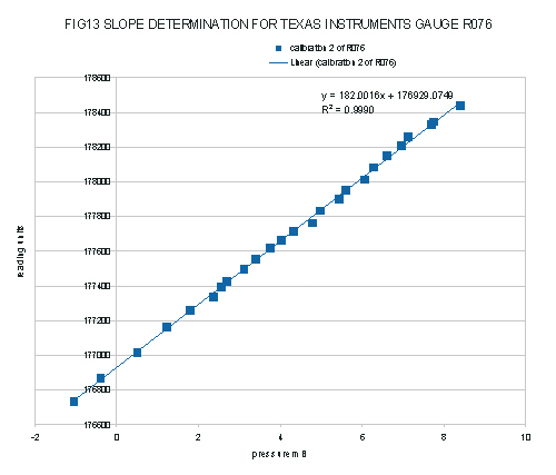
The least square regression shows a slope of 182.0016 counts per millibar to 4 decimal places. In consideration of the errors of the calibration, this should be expressed as 182.0 +/- 0.1 counts per millibar
The second stage of the calibration process was carried out using the apparatus of figure 14. A glass flask of approximately 500ml capacity was suspended in a stirred water bath controlled by a temperature controller R. The temperature of the bath could be measured using a type K thermocouple with an ice/water reference F using a Time Electronics Potentiometer with a resolution of 1 microvolt.
Initially, before connecting the flask V to the Pressure Gauge G, the flask and bath were brought to a temperature of about 80 deg C. The connection between V and G was then made with a fine bore tube (0.25mm bore). The apparatus was allowed to equilibrate at a series of temperatures between 25 and 80 deg C, and at each temperature ( carefully measured using the potentiometer) the reading on the gauge was noted. Care was taken to allow sufficient time for the equilibration to take place in each case.
TABLE 2 - CALIBRATION DATA FOR THE DETERMINATION OF THE INTERCEPT.
| TIME | K ThermEMF mV | Temp deg K | R076 RDNG | PRESSURE | CORRECTED READING |
| 0.590277778 | 2.993 | 346.2805092 | 176412 | 846.1121845 | 153926 |
| 0.597222222 | 2.796 | 341.4483149 | 174302 | 834.305056 | 151816 |
| 0.600694444 | 2.859 | 342.9931814 | 174976 | 838.0798293 | 152490 |
| 0.604861111 | 2.719 | 339.5607373 | 173461 | 829.6928922 | 150975 |
| 0.606944444 | 2.759 | 340.5412151 | 173902 | 832.0886211 | 151416 |
| 0.613888889 | 2.547 | 335.3467387 | 171658 | 819.3962818 | 149172 |
| 0.618055556 | 2.624 | 337.2328217 | 172423 | 824.0047935 | 149937 |
| 0.622916667 | 2.477 | 333.6327132 | 170884 | 815.2081804 | 148398 |
| 0.625 | 2.527 | 334.8569589 | 171404 | 818.1995392 | 148918 |
| 0.631944444 | 2.407 | 331.9192626 | 170057 | 811.0214838 | 147571 |
| 0.633333333 | 2.456 | 333.1186173 | 170483 | 813.952023 | 147997 |
| 0.636805556 | 2.331 | 330.0596045 | 169203 | 806.4775394 | 146717 |
| 0.642361111 | 2.346 | 330.4265874 | 169384 | 807.3742366 | 146898 |
| 0.65 | 2.248 | 328.0294574 | 168314 | 801.5170171 | 145828 |
| 0.65625 | 2.308 | 329.49695 | 169193 | 805.1027325 | 146707 |
| 0.664583333 | 2.162 | 325.9268195 | 167601 | 796.3793685 | 145115 |
| 0.666666667 | 2.184 | 326.4646169 | 167780 | 797.6934388 | 145294 |
| 0.673611111 | 2.094 | 324.2649165 | 166816 | 792.3186249 | 144330 |
| 0.684722222 | 2.008 | 322.1639275 | 165862 | 787.1850054 | 143376 |
| 0.694444444 | 1.934 | 320.3568495 | 165038 | 782.7695367 | 142552 |
| 0.704861111 | 1.848 | 318.2576127 | 164062 | 777.6401986 | 141576 |
| 0.716666667 | 1.77 | 316.354481 | 163210 | 772.9900296 | 140724 |
| 0.729166667 | 1.704 | 314.7447591 | 162446 | 769.0567868 | 139960 |
| 0.739583333 | 1.619 | 312.6724773 | 161538 | 763.9933112 | 139052 |
| 0.75 | 1.546 | 310.893518 | 160700 | 759.6465486 | 138214 |
| 0.750694444 | 1.54 | 310.7473337 | 160640 | 759.2893577 | 138154 |
| 0.753472222 | 1.539 | 310.7229702 | 160606 | 759.229827 | 138120 |
| 0.763888889 | 1.488 | 309.4806057 | 160040 | 756.1941964 | 137554 |
| 0.76875 | 1.437 | 308.2385907 | 159500 | 753.1594196 | 137014 |
| 0.775 | 1.396 | 307.2403623 | 159040 | 750.7203186 | 136554 |
The data in table 2 was processed and derived as follows:
(a) the EMF values in column 2 were converted to degrees K using the equation:
![]()
where v = thermocouple voltage in volts, and an= coefficients as defined in Table 3:
The procedure followed produced a useful absolute calibration of a precision instrument for pressure measurement. The key
quantity upon which the precision of the whole procedure rests is that of the slope determined in table 1. This has an estimated accuracy of 0.1 in 182, limited
by the fact that the travelling microscope only had a 20cm useful travel. Using a longer instrument with a larger range of manometric heights
would resulted in a greater precision in the final result.
The use of an enclosed gas volume at a known temperature as an absolute pressure reference worked very well as a
calibrating method and the calibration obtained can be relied upon to an accuracy of 0.1mB overall.
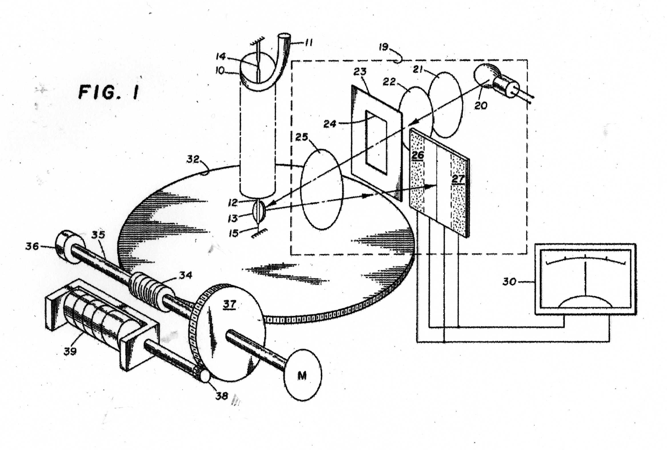
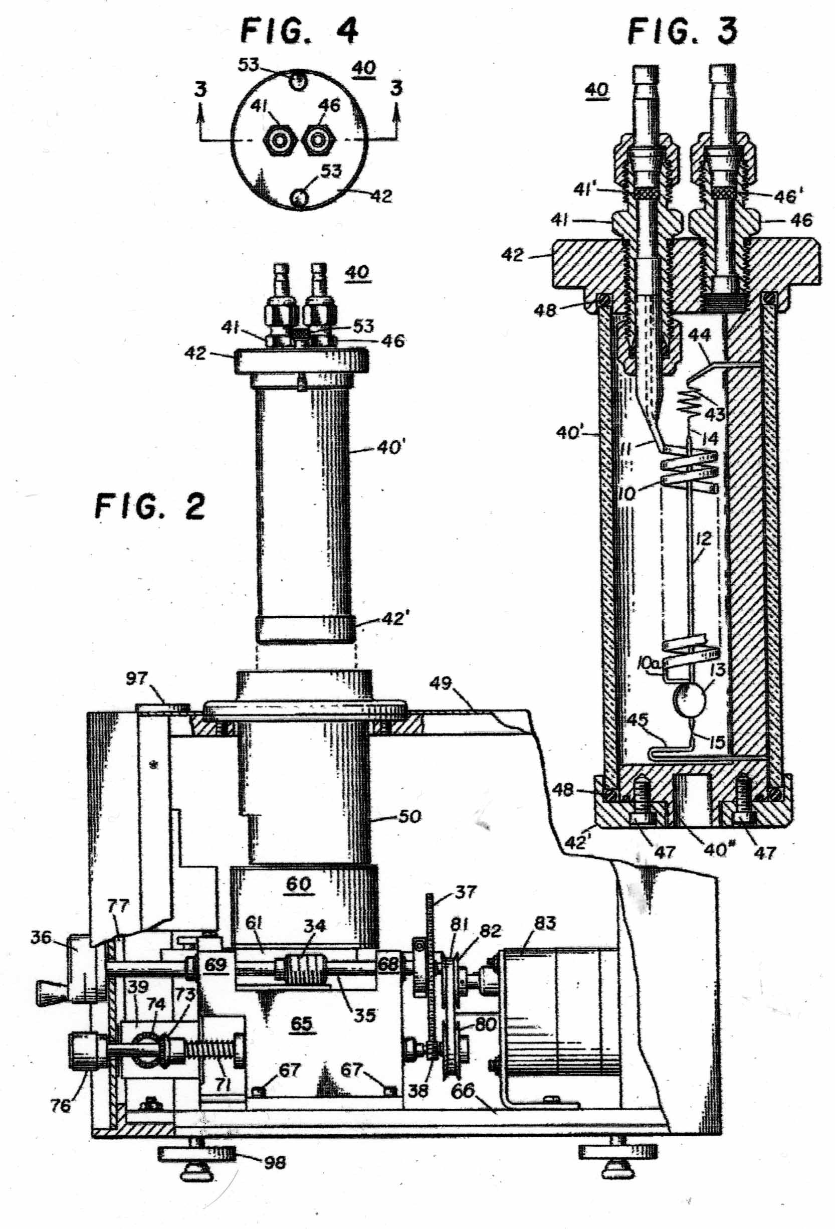
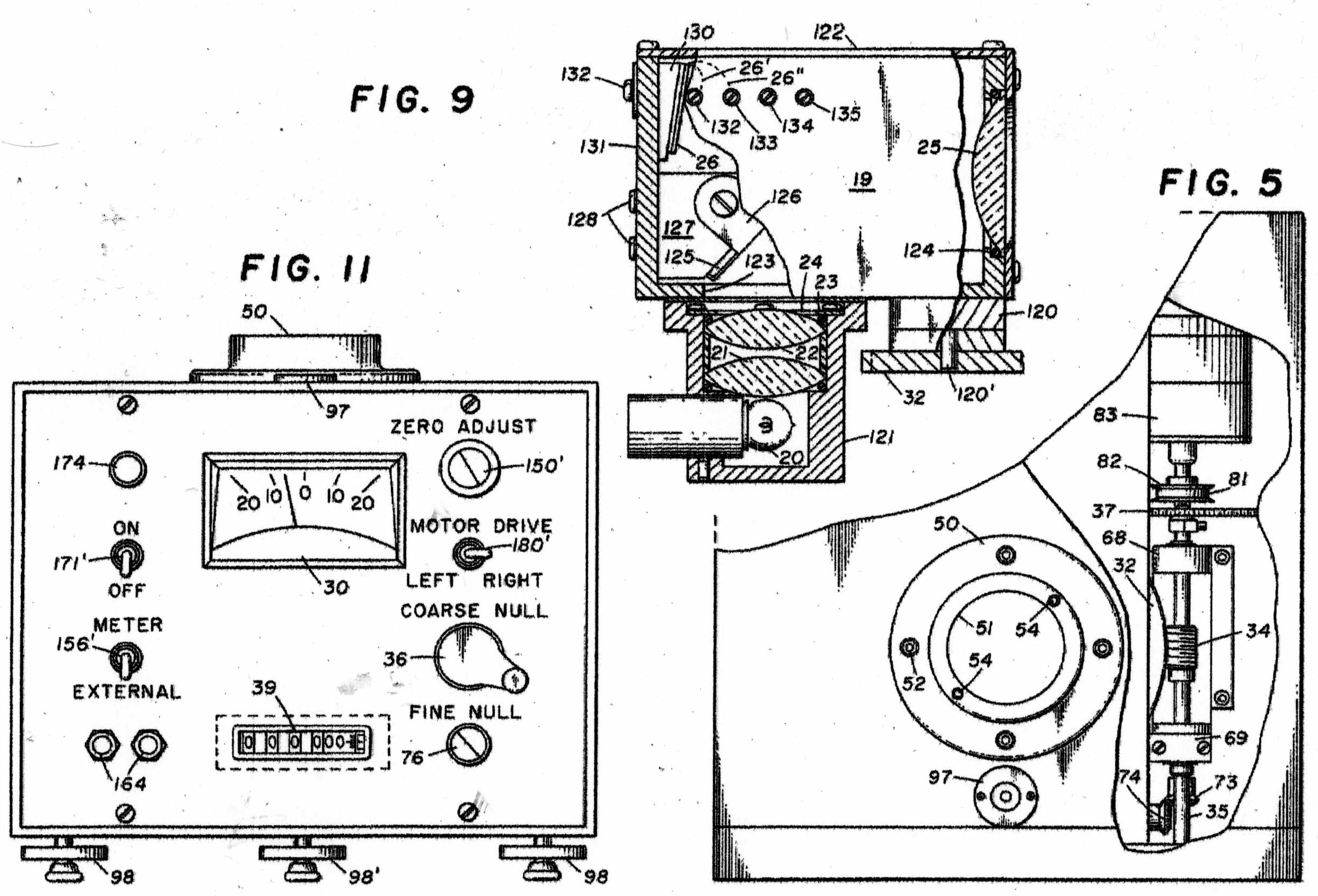
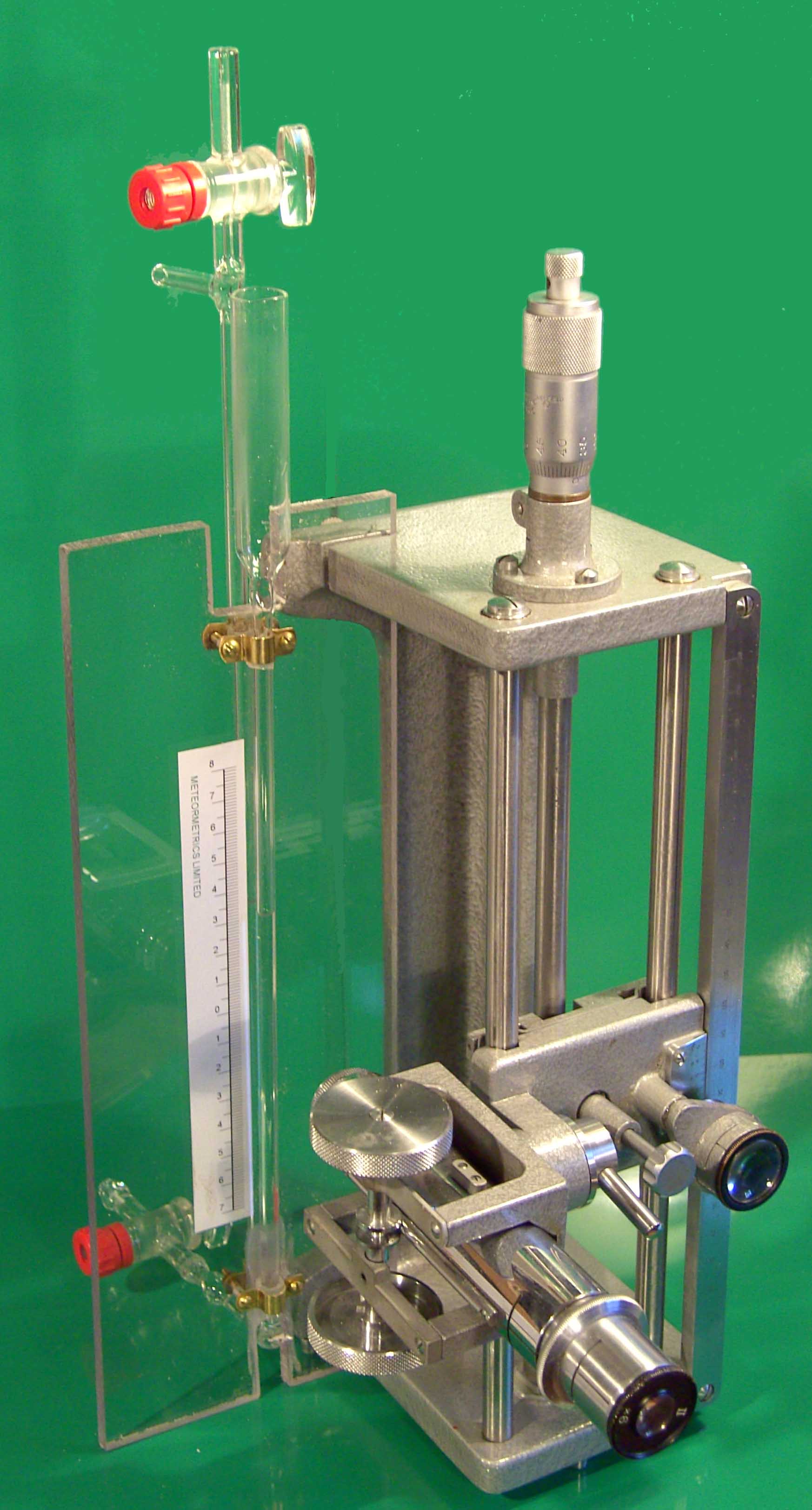
Figure 12, A water manometer mounted on a vertical travelling microscope used for the slope determination.
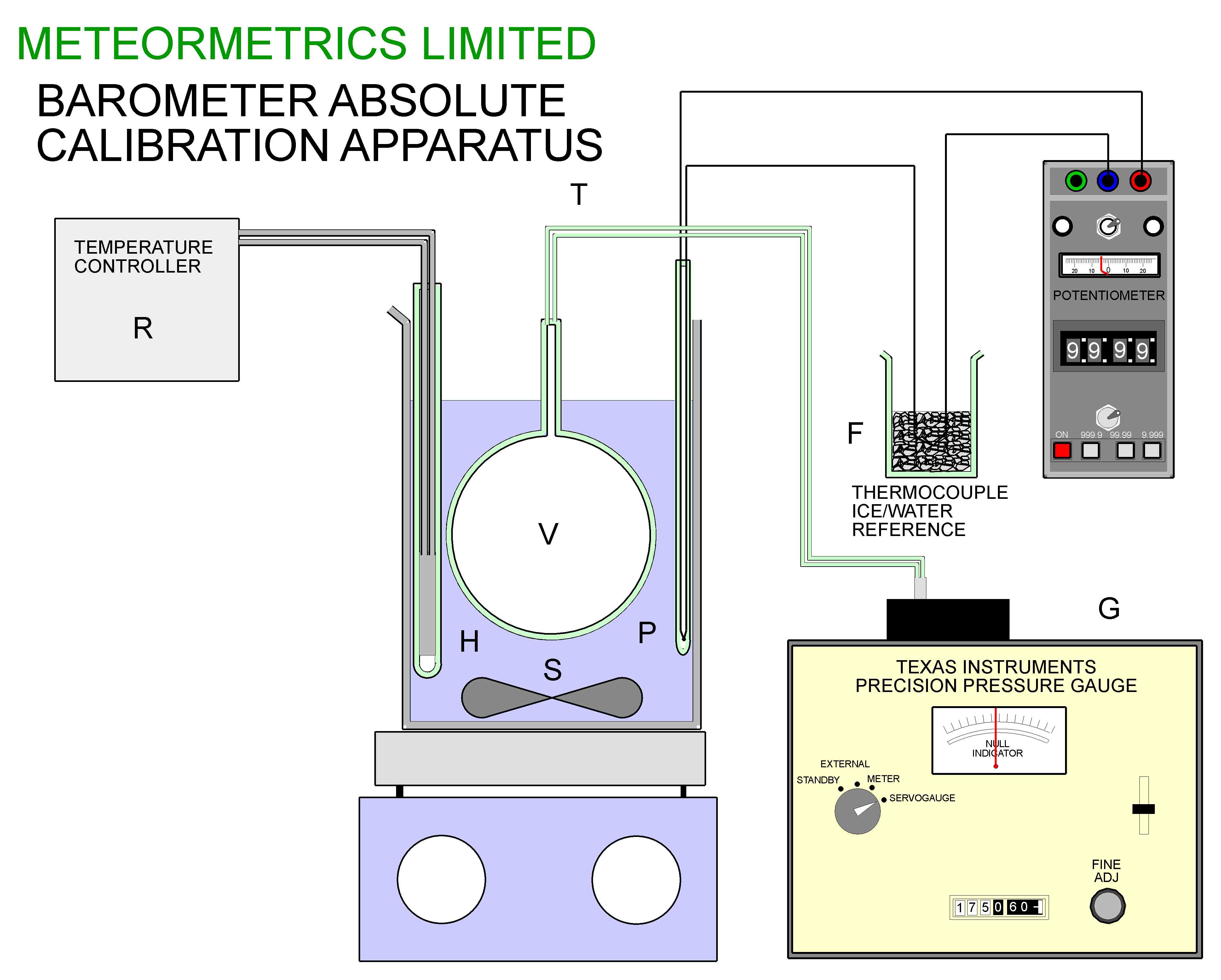
Figure 14, The apparatus for determining the intercept and final calibration
| n | an |
| 0 | 0.2265846 |
| 1 | 24152.1090000 |
| 2 | 67233.4248000 |
| 3 | 2210340.6820000 |
| 4 | -860963914.9000000 |
| 5 | 48350600000.0000000 |
| 6 | -1184520000000.0000000 |
| 7 | 13869000000000.0000000 |
| 8 | -63370800000000.0000000 |
Table 3, Coefficients of polynomial for K type thermocouples
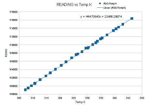
Figure 15, Plot of pressure gauge reading against absolute temperature
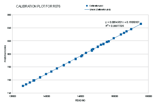
Figure 16, The final absolute calibration plot obtained for the Texas Instruments, Precision Pressure Gauge.